The Intelligence Layer: ML Anomaly Detection, Drift, and Alert Auto-Tuning

Synthetic Monitoring Series — Part 8
The Intelligence Layer: ML Anomaly Detection, Drift, and Alert Auto-Tuning
If your team has learned to ignore alerts, your monitoring is worse than useless. It’s providing false confidence. Alert fatigue is one of the most corrosive problems in operations — and it almost always starts with static thresholds.
This post covers the three techniques that replace static thresholds with learned behavior: anomaly detection that understands time-of-day patterns, change-point and drift detection that catch gradual degradation, and alert auto-tuning that reduces noise while preserving every genuine signal.
Start Here: What the Videos Cover
▶ Video 21 — “ML Anomaly Detection — Beyond Static Thresholds”
▶ Video 22 — “Change-Point and Drift Detection — Catching the Slow Burn”

▶ Video 23 — “Alert Auto-Tuning and Flapping Detection”

Why Static Thresholds Fail
Static thresholds ask a single question: is this value too high? That sounds reasonable until you watch it fail in practice.
The Problem | The Solution |
|---|---|
Static Threshold at 500ms | ML-Learned Threshold |
Normal daily peak at noon pushes latency to 510ms — false alert fires. At 3 AM, a genuine anomaly pushes latency to 300ms — well below the threshold, but completely abnormal for that hour. Missed entirely. | At noon, 480ms is expected — no alert. At 3 AM, anything above 120ms is suspicious — alert fires. The threshold follows the metric’s natural rhythm instead of a fixed line drawn by a human guess. |
The deeper problem with static thresholds is that they require constant manual maintenance. Traffic patterns change with seasons, product launches, and user growth. A threshold that was well-tuned six months ago is wrong today — and most teams don’t update them until they’ve been burned by enough false positives or missed incidents to force a review.
ML Anomaly Detection: Is This Value Unusual Right Now?
ML anomaly detection asks a better question than “is this value too high?” It asks: is this value unusual for this time of day, this day of week, given what’s been normal for this metric over the past weeks?
The algorithm used for this is Isolation Forest. It works by randomly partitioning the data space. Normal data points require many cuts to isolate — they’re surrounded by similar values. Anomalies require few cuts — they’re outliers, easy to separate from the rest of the distribution. The fewer cuts required, the higher the anomaly score.
Sensitivity configuration
Sensitivity Level | Behavior | Best For |
|---|---|---|
High | Catches subtle shifts; may fire during planned deployments | Critical endpoints where early warning outweighs noise |
Medium (default) | Balanced; ignores minor variation, catches meaningful deviations | Most production monitoring |
Low | Only triggers on dramatic deviations; very low false positive rate | High-volume services where noise tolerance is low |
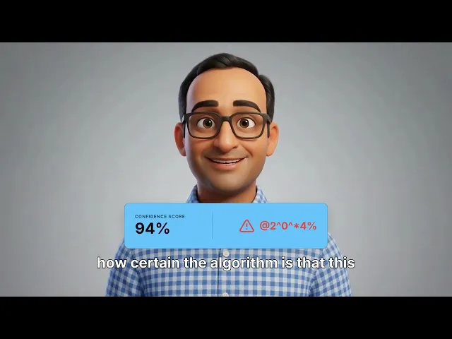
Each detection also includes a confidence score — how certain the algorithm is that this is a real anomaly. High-confidence detections are immediately actionable. Lower-confidence detections are flagged for review rather than triggering a page.
Change-Point and Drift Detection: Catching What Spikes Can’t
Anomaly detection catches spikes — sudden deviations that resolve quickly. But two other failure patterns are equally common and harder to detect: step changes that shift a metric permanently to a new level, and gradual drift that accumulates over weeks or months without any single measurement looking wrong.
The Drift Problem
Your baseline DNS resolution time was 30ms six months ago. Today it’s 45ms. No single measurement triggered an anomaly. No step change is visible. But the cumulative drift is 50% — and it’s quietly eating into your latency budget while every check says “normal.”
Change-point detection: the PELT algorithm
Change-point detection identifies the exact moment a metric’s behavior permanently shifts. The PELT algorithm — Pruned Exact Linear Time — analyzes the statistical properties of the data on either side of every possible cut point. When a cut produces two segments with significantly different means or variances, that’s a change point. The result: you see not just that something changed, but exactly when, expressed as a timestamp.
Drift tracking
Drift tracking measures gradual divergence from a learned baseline. Rather than comparing each measurement to an absolute threshold, it compares the current rolling average to the historical baseline and fires when the accumulated drift exceeds a configured percentage — typically 10-20% for most metrics.
Alert Auto-Tuning and Flapping Detection
Even with ML-based detection, alerting systems accumulate noise over time. Thresholds that were well-positioned become misaligned as systems change. The most common symptom is flapping — an alert that fires and resolves dozens of times per hour because the threshold sits too close to the metric’s normal operating range.
How flapping detection works
The system counts state transitions — alert fires, alert resolves, alert fires again — within a rolling time window. Twelve state changes in one hour indicates a flapping alert. Rather than continuing to page the on-call team twelve times per hour, the system identifies the threshold as misaligned and suppresses further alerts while flagging it for review.
Auto-tuning: suggest, don’t decide
Auto-tuning analyzes the historical distribution of the metric relative to the current threshold and calculates a better position. Moving a threshold from the 50th percentile to the 95th percentile of normal values converts a threshold that fires constantly into one that fires only when something genuinely unusual happens.
Auto-tune suggests. Humans decide.The algorithm understands the math. You understand the business context — whether a 95th percentile threshold is aggressive enough for a payment endpoint, or too conservative for an internal service. Both inputs are necessary. |
|---|
~70% | Reduction in alert volume achievable with proper auto-tuning — while catching every genuine incident. Less noise. More signal. Teams that trust their alerts respond faster. | |
The Three Pillars: Every Way a Metric Can Go Wrong
⚡ | → | ↗ |
|---|---|---|
Anomaly Detection | Change-Point Detection | Drift Tracking |
Catches sudden spikes and unexpected values relative to learned time-of-day patterns. | Identifies the exact moment a metric permanently shifts to a new operating level. | Measures cumulative divergence from a learned baseline over days, weeks, or months. |
Together, these three techniques cover every mode of metric degradation. A spike that resolves in minutes. A permanent step change after a deployment. A gradual creep that takes six months to become a problem. No single detection method catches all three — but all three together leave nowhere for a problem to hide.
Next in the Series
Part 9 — Putting It All Together: A Synthetic Monitoring Strategy. A complete, production-ready monitoring architecture built from the ground up — probes, protocols, intervals, ML detection, and alert escalation.
ML Anomaly DetectionAlert Auto-TuningDrift DetectionChange-Point DetectionAlert FatigueAIOpsSynthetic MonitoringSREInfrastructure Observability
About Parlon
Parlon is an infrastructure observability platform built for enterprise teams operating complex, hybrid environments. Parlon combines active synthetic validation, real-time telemetry normalization, and learning-based alerting into a single platform — shifting operations from firefighting to foresight. Learn more at parlon.io.