Probe Architecture, P2P Testing, and Path Intelligence

Synthetic Monitoring Series — Part 7
Probe Architecture, P2P Testing, and Path Intelligence
External checks tell you if the internet is working. Probe-to-probe checks tell you if your network is working. That’s a fundamentally different — and often more valuable — question.
This post covers three interconnected topics that together define how production-grade synthetic monitoring is actually built and deployed: how probes are architected to survive the outages they’re designed to catch, how probe-to-probe testing reveals what external monitoring can’t see, and how to locate exactly where a bottleneck lives on a network path.
Start Here: What the Videos Cover
▶ Video 17 — “Probe Architecture — Resilience at the Edge”
▶ Video 18 — “Probe-to-Probe Testing — Measuring Your Own Network”
▶ Video 19 — “Path Bandwidth Discovery — Finding the Bottleneck”

▶ Video 20 — “Unified Traceroute — Continuous Path Intelligence”
Probe Architecture: Built to Survive the Outage
There’s a paradox at the heart of monitoring architecture: the worst time for your monitoring system to fail is during an outage. If the probe stops collecting data the moment the network goes down, you lose exactly the data you need most — the measurements from the incident itself.
Edge-first probe design solves this. Rather than waiting for instructions from a central server, the probe uses a pull model: it asks the central server for work. If the server becomes unreachable, the probe doesn’t stop — it keeps executing its scheduled checks and caches results locally until connectivity returns.
The probe lifecycle
1 | Registration Probe registers with the central API and receives a unique ID. Configuration is pulled, not pushed. |
2 | Heartbeat & Task Poll Every 30 seconds, the probe polls for task assignments. This doubles as a heartbeat — silence from a probe triggers an alert. |
3 | Check Execution Assigned checks run on schedule. Results are generated locally — the probe doesn’t need the central server to execute a check. |
4 | Local Caching Results are stored in a local cache. If connectivity to the API is lost, results accumulate locally without data loss. |
5 | Batch Submission Results are submitted in compressed batches when connectivity is available. After an outage, the full incident data arrives in a burst — complete coverage through the entire event. |
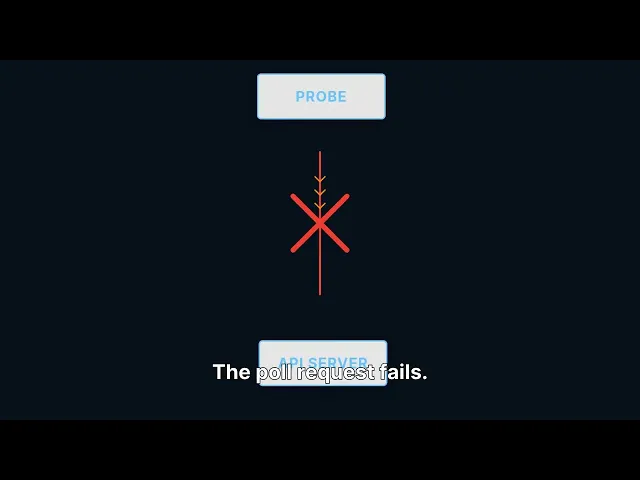
WHAT HAPPENS IN AN OUTAGE | ||
|---|---|---|
T+0:00 | Network connectivity between probe and API server breaks. Poll request fails. | |
T+0:30 | Probe continues all scheduled checks. Results cached locally. No data lost. | |
T+8:00 | Connectivity restores. Probe immediately submits cached results in compressed batch. | |
T+8:01 | Complete measurement data available for the entire 8-minute incident window — exactly when you need it most. | |
Probe-to-Probe Testing: Measuring the Network You Own
External checks measure how your service looks to the outside world. They tell you whether users can reach your application and how fast it responds. What they cannot tell you is how your internal network is performing — the WAN links between offices, the cloud interconnects between regions, the paths that only internal traffic uses.
Probe-to-probe (P2P) testing measures those paths directly. Two probes send test traffic to each other and measure the result. Because you control both endpoints, you can measure the paths that external checks can’t reach.
The four P2P metrics
Metric | Why Direction Matters |
|---|---|
Bidirectional RTT | Measured independently in each direction — asymmetric routing means NY→London and London→NY often differ by measurable amounts |
Jitter | Variation in latency; 10ms of jitter on a VoIP call produces choppy audio even if average latency is acceptable |
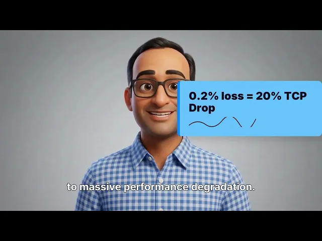
Packet loss | Even 0.1% loss degrades TCP throughput significantly; P2P testing catches this continuously on paths that external checks never see |
Throughput | Maximum achievable data rate, measured using RFC 2544 methodology on real network paths |
Real-World Scenario
VoIP calls between your New York and London offices sound choppy. External checks are all green — the internet is fine. A P2P test between your New York and London probes reveals 2% packet loss on your WAN link. That’s your answer — and no external check would ever find it, because external checks don’t run on the paths you own and operate.
Path Bandwidth Discovery: Finding the Exact Bottleneck
Every other tool tells you the path is slow. Path Bandwidth Discovery tells you that hop 3 is a 100-megabit link bottlenecking your gigabit path. That’s the difference between knowing there’s a problem and knowing exactly what to fix.
The Variable Packet Size (VPS) algorithm exploits a basic law of physics: serialization delay — the time it takes to push a packet onto a link — is directly proportional to packet size divided by link speed. A larger packet takes proportionally longer to transmit on a slower link.
By sending two packets of different sizes to the same hop and measuring the time difference, PBD can calculate the serialization rate, which directly reveals the link’s bandwidth. The formula is: capacity equals eight divided by the slope of the delay-versus-size curve. The result is a per-hop bandwidth map of the entire path.
What a bandwidth map looks like
Hop | Estimated Capacity | Confidence | Status |
|---|---|---|---|
Hop 1 | 1,000 Mbps | High | Normal |
Hop 2 | 1,000 Mbps | High | Normal |
Hop 3 | 100 Mbps | High | ⚠ Bottleneck |
Hop 4 | 1,000 Mbps | Medium | Normal |
Plain traceroute tells you the path. Path Bandwidth Discovery tells you the capacity at every point along it. Traceroute is a road map. PBD is a traffic report with speed limits marked for every segment.
Continuous Traceroute: From Diagnostic Tool to Early Warning System
Running traceroute manually when something is broken is like checking your tire pressure after the flat. By the time you run it, the routing change that caused the problem may already be gone, replaced by a new path that looks healthy.
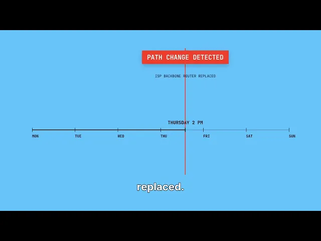
Continuous traceroute runs automatically — every 60 seconds, from every probe. Each session records the full hop sequence with per-hop RTT and packet loss. The path is hashed with SHA-256. If any router in the path changes, the hash changes, and an alert fires immediately — without anyone manually comparing hop sequences.
Hash the path. Compare continuously. Alert on change. Monday through Wednesday the hash is consistent. Thursday at 2 PM the hash changes — a router in your ISP’s backbone was replaced or rerouted. You see the exact moment it happened, without anyone filing a ticket or noticing degraded performance first.
Per-hop loss identification adds another layer. If hop 5 shows 2.3% packet loss while every other hop is at zero, you know exactly where packets are being dropped. Not “somewhere between New York and London” — but at a specific router, at a specific moment, with a timestamp.
Next in the Series
Part 8 — The Intelligence Layer: ML Anomaly Detection, Drift, and Alert Auto-Tuning. How machine learning moves alerting from static thresholds to learned behavior — and why that changes everything about operational noise.
Synthetic MonitoringProbe ArchitectureP2P TestingPath Bandwidth DiscoveryContinuous TracerouteWAN MonitoringNetwork ObservabilitySRE
About Parlon
Parlon is an infrastructure observability platform built for enterprise teams operating complex, hybrid environments. Parlon combines active synthetic validation, real-time telemetry normalization, and learning-based alerting into a single platform — shifting operations from firefighting to foresight. Learn more at parlon.io.